Chapter 1 Introduction
“…while we take it for granted that sounds may be described visually, the convention is recent, is by no means universal and, as I will show, is in many ways dangerous and inappropriate.”
While Murray Schafer’s Tuning of the World (Schafer 1977) inspired many soundscape scientists, this view is of an earlier time when the concept of multiple simultaneous streams of acoustic data processed in real time by a single entity was still an idea beyond the horizon. Individual sounds could be isolated and studied (as today they still are by bioacousticians interested in the behaviour of individual species). The scale of many contemporary ecoacoustics projects precludes an individual from listening to every minute recorded; the task is no longer delegated to students but to networks of machines.
Additionally, it is now helpful to distinguish between two concepts that Schafer bought together under the concept of notation. That is to separate notation (phonetics and musical notation) from visual representations of the physical properties of acoustic waves (e.g. amplitude, frequency).
Historically, researchers used musical notation and phonemes to describe the songs of various animals. However, these methods do not scale to the entirety of the natural soundscape. Parts of the soundscape are beyond the limits of human hearing; the infrasound, the ultrasound, and the quiet. All manner of information is gathered and shared by other species beyond the limits of our perception. Visualisation is the primary tool by which we can interpret the entire soundscape for all species that share it.
1.2 Basic acoustic concepts
A sound wave is a disturbance in the air that propagates as a series of compressions (the regions between are known as regions of rarefaction), see Figure 1.1. The frequency of a sound wave is the number of compressions and rarefactions that pass a point in a second. The amplitude of a sound wave is the difference between the maximum and minimum pressure of the wave.
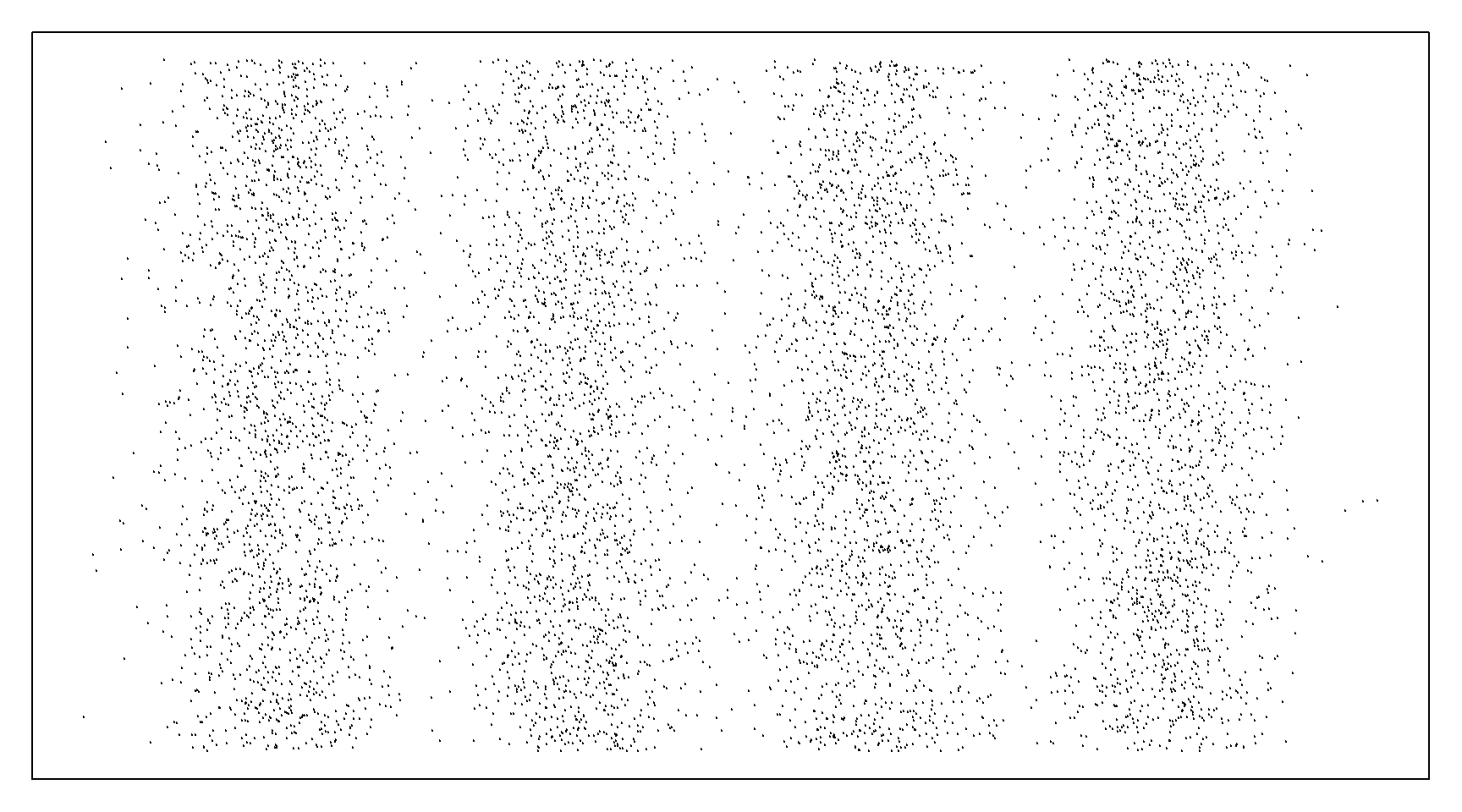
Figure 1.1: A wave in air.
1.3 Types of files
Even though the costs of digital storage have fallen significantly (Figure 1.2), the cost of file transfer and storage are still significant factors in many acoustics projects. For this reason, it is sometimes necessary to compress the audio file in some way: discarding some data in exchange for cost reductions.
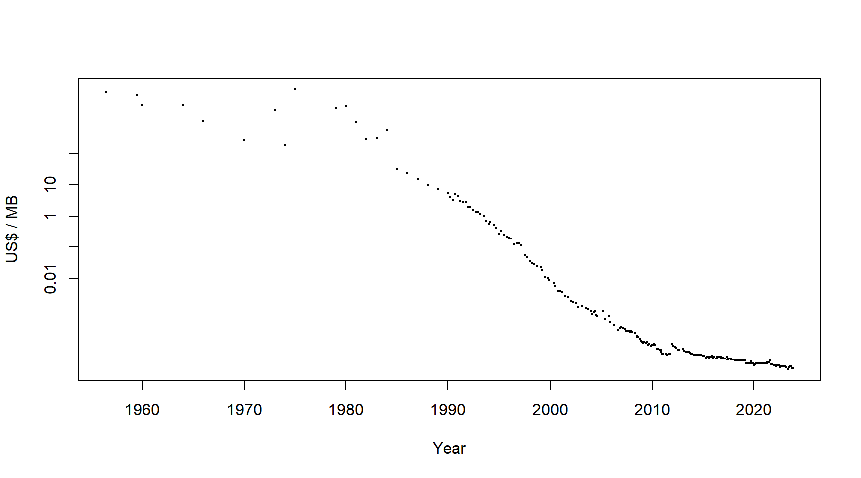
Figure 1.2: Storage costs per megabyte over time. Data from https://jcmit.net/diskprice.htm.
This process of compression may affect the visualisation of the audio files or even the possible types of visualisation for a given file.
1.3.1 Uncompressed waveform files
Waveform files are created by sampling the wave amplitude at a sensor at a constant rate, typically tens of thousands of times per second (Figure 1.3).
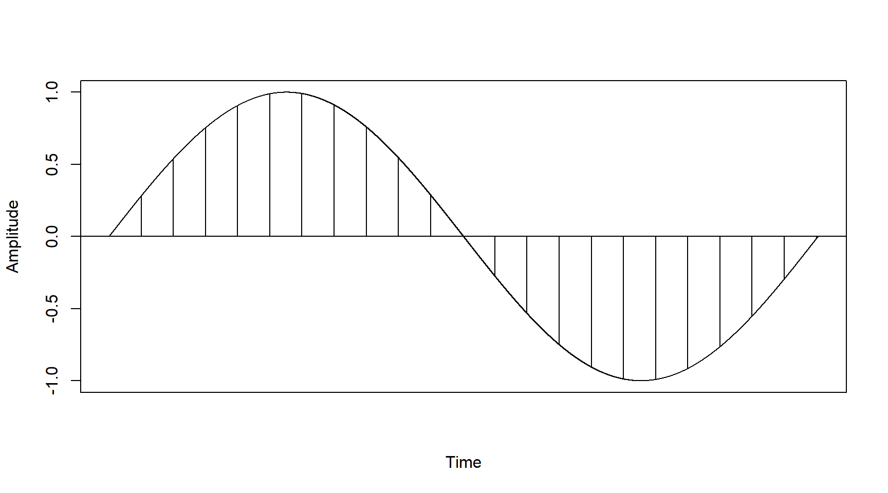
Figure 1.3: Sampling a waveform.
An analogue-to-digital converter (ADC) converts the continuous variations in amplitude into one of the numerous discrete levels that the ADC can represent (Figure 1.3. The number of discrete levels is dependent on the analogue-to-digital converter (ADC); a typical 16-bit depth has \(2^{16}=65536\) possible values.
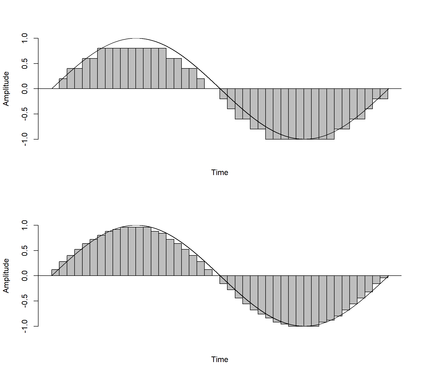
Figure 1.4: A sampled waveform with low bit depth (top) and higher bit depth(bottom).