Chapter 7 Patterns of activity

Many organismal activities are tied to the cycles of the day, particularly in temperate zones, cycles of the year. These cycles bring regular fluctuations in light levels, day lengths, temperatures, and various other influences. Often these cycles interact, with the dawn chorus peaking in the early daylight hours and its timing and intensity fluctuating on a yearly cycle. This chapter looks at visualising these cycles and the effects of lunar cycles.

These plots are created using the SonicScrewdriver package (Baker 2021), which uses the suncalc package (Thieurmel and Elmarhraoui 2019) to perform the required sun and moon position calculations. The Plotrix package (Lemon 2006) is used for creating the visualisation. These packages are installed as shown below.

install.packages(c("plotrix", "sonicscrewdriver"))

The SonicScrewdriver package must be loaded before constructing a visual.

library(sonicscrewdriver)

7.1 Daily Cycles

Broughton (1963) contests the term diel for daily cycles as an incorrectly formed, unnecessary neologism. However, it sees greater use (according to the online Oxford English Dictionary) than his suggested nycthemeral.

The design for these plots came from a desire to compare the dawn chorus at various locations around the UK. However, they also offer great potential for comparing locations with greater longitudinal or latitudinal separation. The plots show the times of day, night, twilight (7.1.1), sunrise, sunset, nadir and solar noon. The day part of the plot shows the altitude (angle of the sun above the horizon) throughout the day, with the maximum value representing the sun directly overhead.

7.1.1 The Types of Twilight

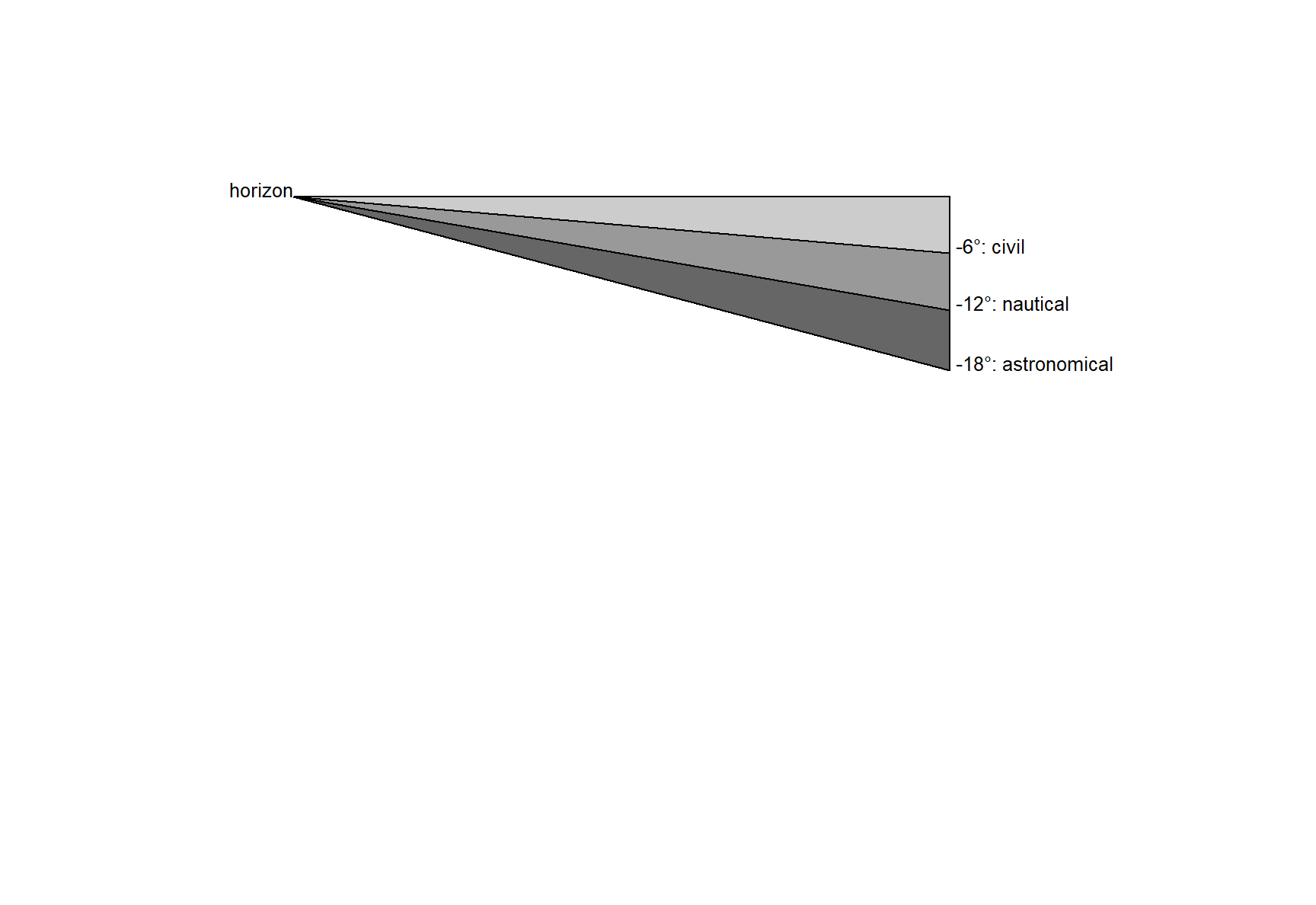
Figure 7.1: Different types of twilight as the sun sets below the horizon

7.1.1.1 Civil Twilight

Civil twilight occurs when the sun’s geometric centre (as seen from Earth) passes between 0° and 6° below the horizon. During this time, it is normal for humans not to need the assistance of artificial light for everyday tasks.

7.1.1.2 Nautical Twilight

Nautical twilight occurs when the sun is between 6° and 12° below the horizon. During this time, there is sufficient light to distinguish the horizon without illumination from the moon (allowing the determination of position at sea through star sightings).

7.1.1.3 Astronomical Twilight

Many astronomical observations are possible when the sun is between 12° and 18° below the horizon. Some light from the sun is visible through the atmosphere. Often considered a dark sky in urban areas with light pollution.

7.1.2 Diel Plots

As the times of the solar day are dependent both on the date and location these must be passed to the dielPlot() function.

dielPlot("2022-08-08", lat=53, lon=0.1)

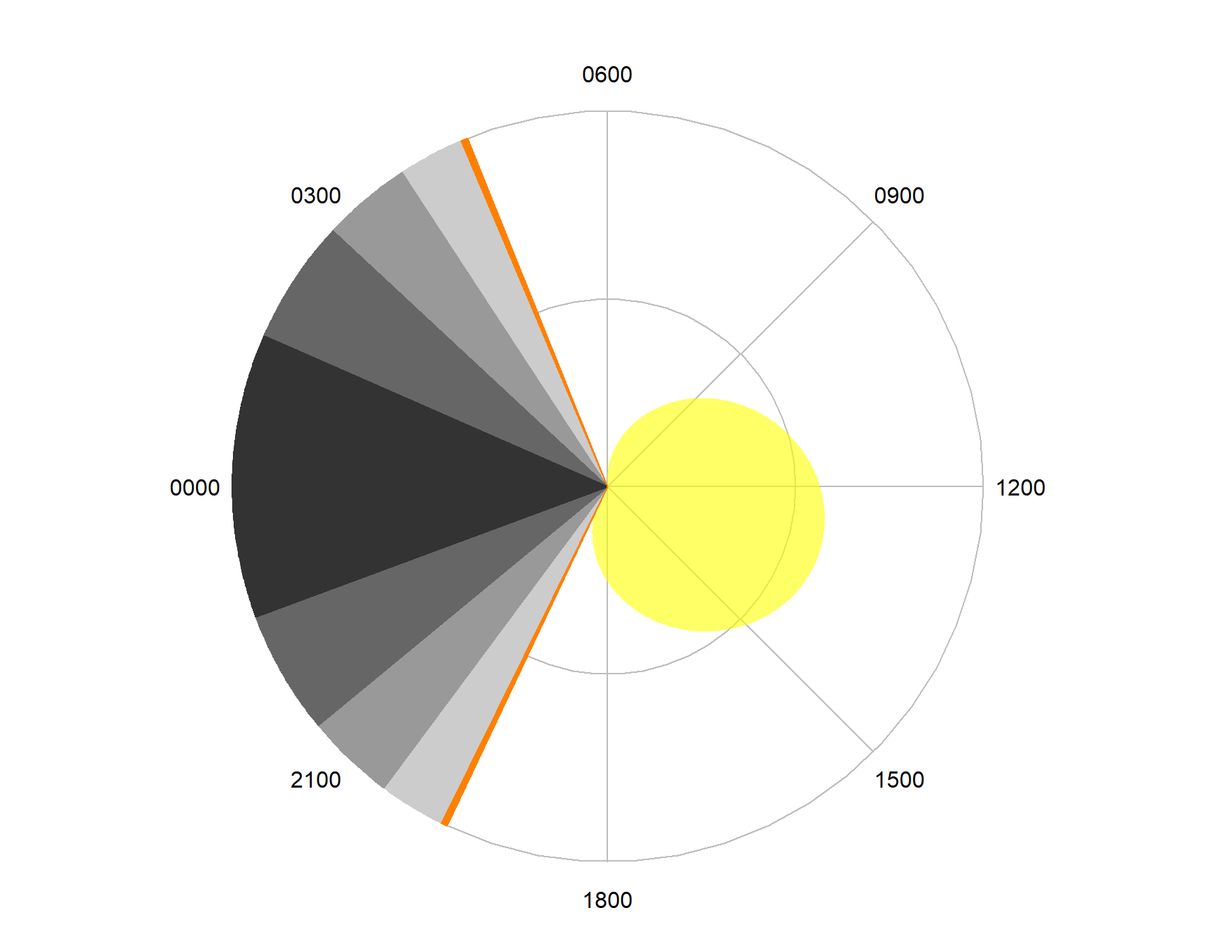
Figure 7.2: Example of a diel plot

7.1.2.1 Rotations of a `dielPlot()`

By default the information is plotted in the UTC timezone, so locations in other timezones will have an overall rotation.

par(mfrow=c(1,3))
dielPlot(Sys.Date(), lat=53, lon=-50)
dielPlot(Sys.Date(), lat=53, lon=-0)
dielPlot(Sys.Date(), lat=53, lon=50)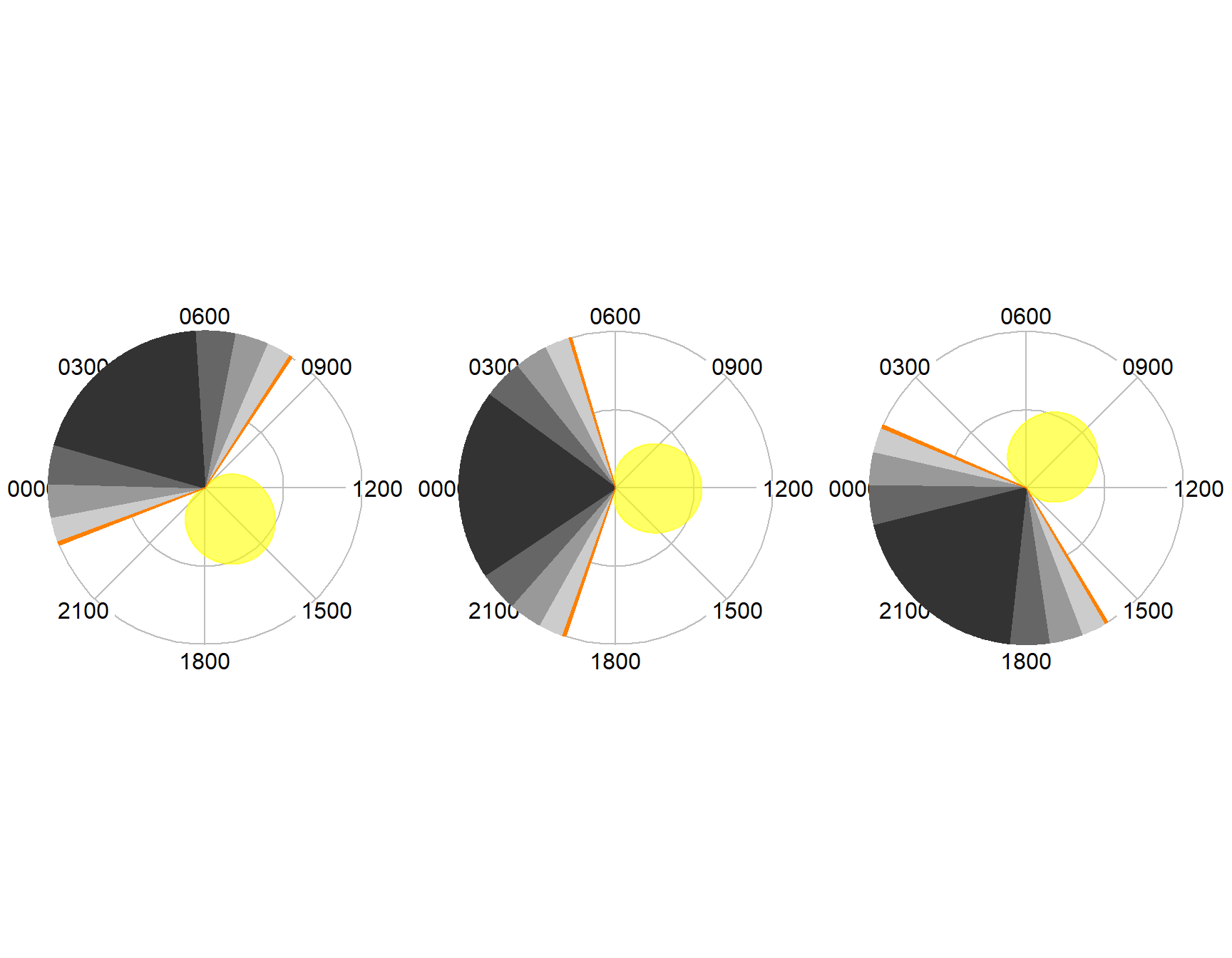

Figure 7.3: Diel plots in UTC.

Plots can be made in any timezone by using the rot parameter to dielPlot() and the tz() function.

par(mfrow=c(1,3))
dielPlot(Sys.Date(), lat=53, lon=-50, rot=tz(3))
dielPlot(Sys.Date(), lat=53, lon=-0, rot=tz(3))
dielPlot(Sys.Date(), lat=53, lon=50, rot=tz(3))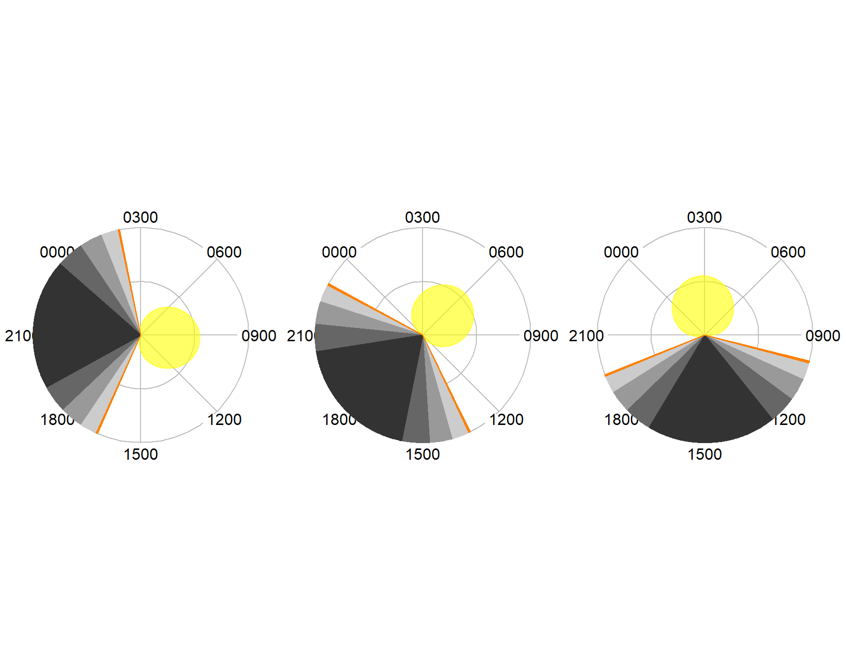

Figure 7.4: The same diel plots in UTC +3

By setting the rot parameter to Solar Noon it is possible to align the plots to solar noon. Notice that this rotates the plot labels.

par(mfrow=c(1,3))
dielPlot(Sys.Date(), lat=53, lon=-50, rot="Solar Noon")
dielPlot(Sys.Date(), lat=53, lon=-0, rot="Solar Noon")
dielPlot(Sys.Date(), lat=53, lon=50, rot="Solar Noon")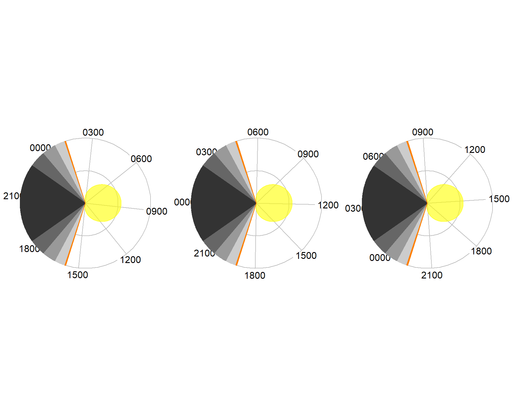

Figure 7.5: The same diel plots aligned to solar noon

7.1.2.2 Customising a `dielPlot()`

In addition to the date, lat and lon parameters to dielPlot() it is possible to make additional customisations to how the information is presented.

Legend

A legend can be added to the plot by setting legend=TRUE.

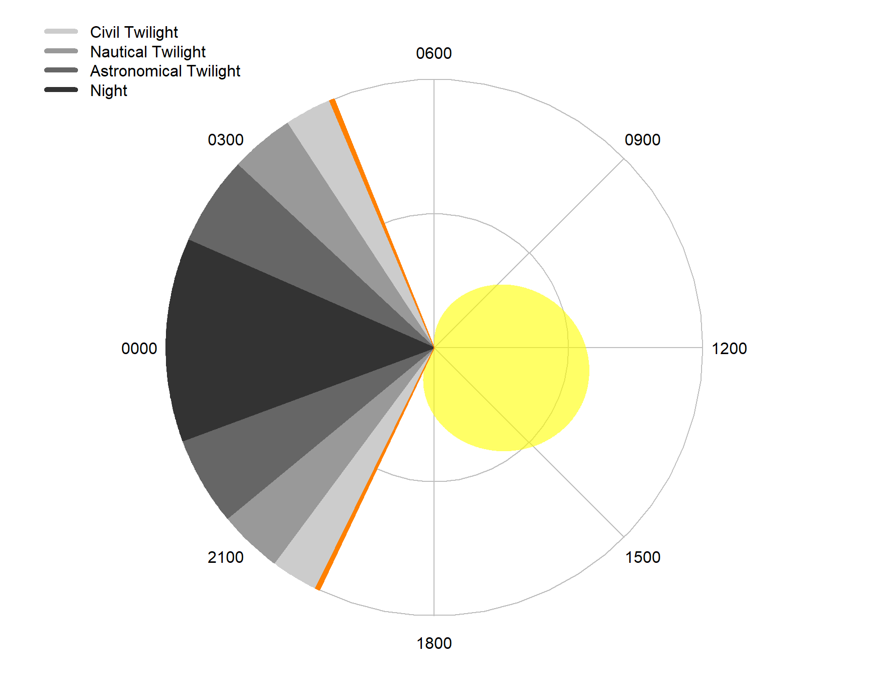
dielPlot("2022-08-08", lat=53, lon=0.1, legend=TRUE)

Figure 7.6: Example adding a legend to a diel plot

Plotting Components

The components that can be plotted are listed below. By default all are plotted except for Solar Noon and Nadir.

Name	Notes
Astronomical Twilight
Nautical Twilight
Civil Twilight
Sunrise
Solar Noon	The time when the sun is highest in the sky
Sunset
Nadir

The components that are plotted can be specified using the plot parameter.

components <- c("Sunrise", "Sunset", "Solar Noon", "Nadir")
dielPlot("2022-08-08", lat=53, lon=0.1, plot=components)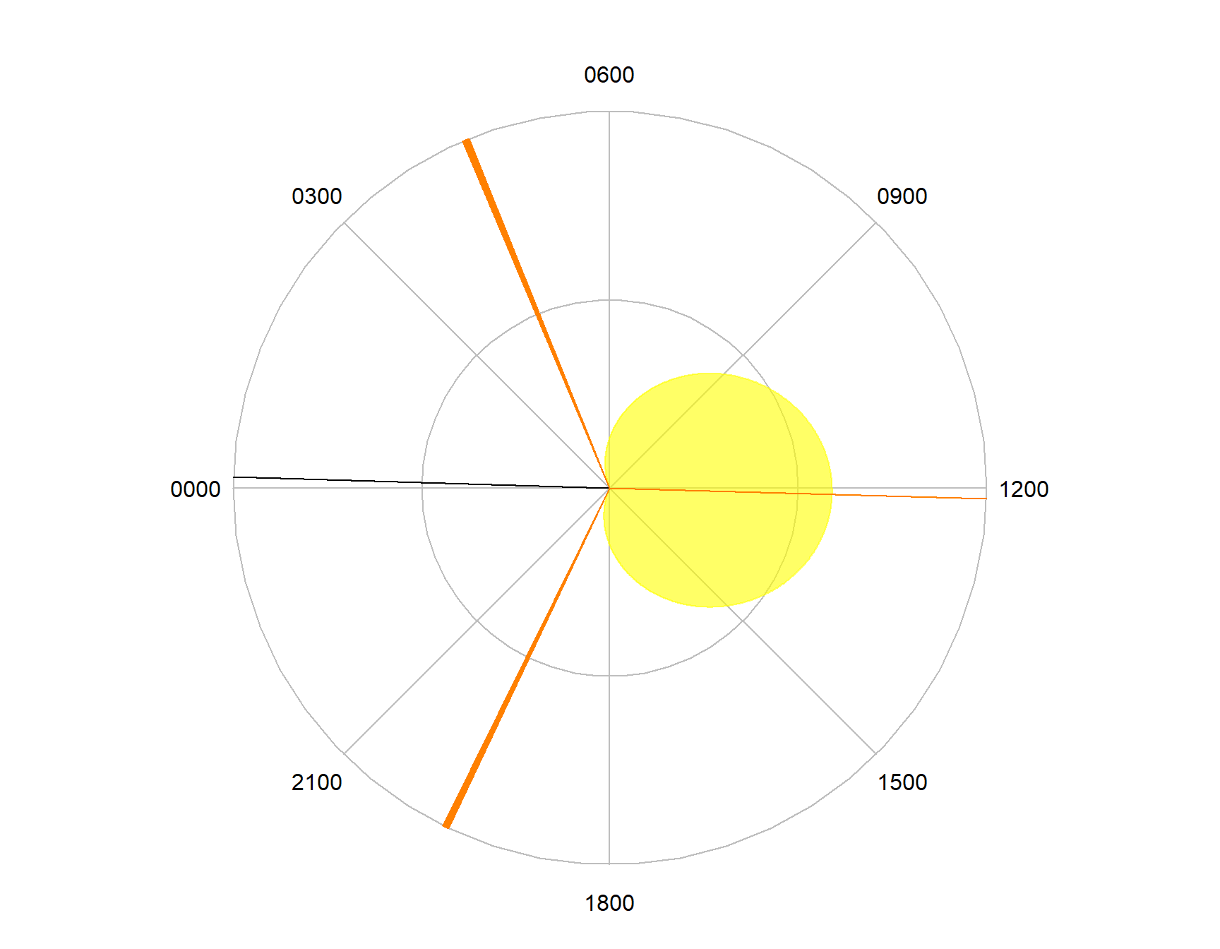

Figure 7.7: Selecting the components to plot

7.2 Yearly Cycles

The yearlyPlot() function from the SonicScrewdriver package shows daylight changes throughout a year. It behaves in a very similar fashion to dielPlot but takes a single year rather a date as input.

yearlyPlot(2022, lat=53, lon=0.1)

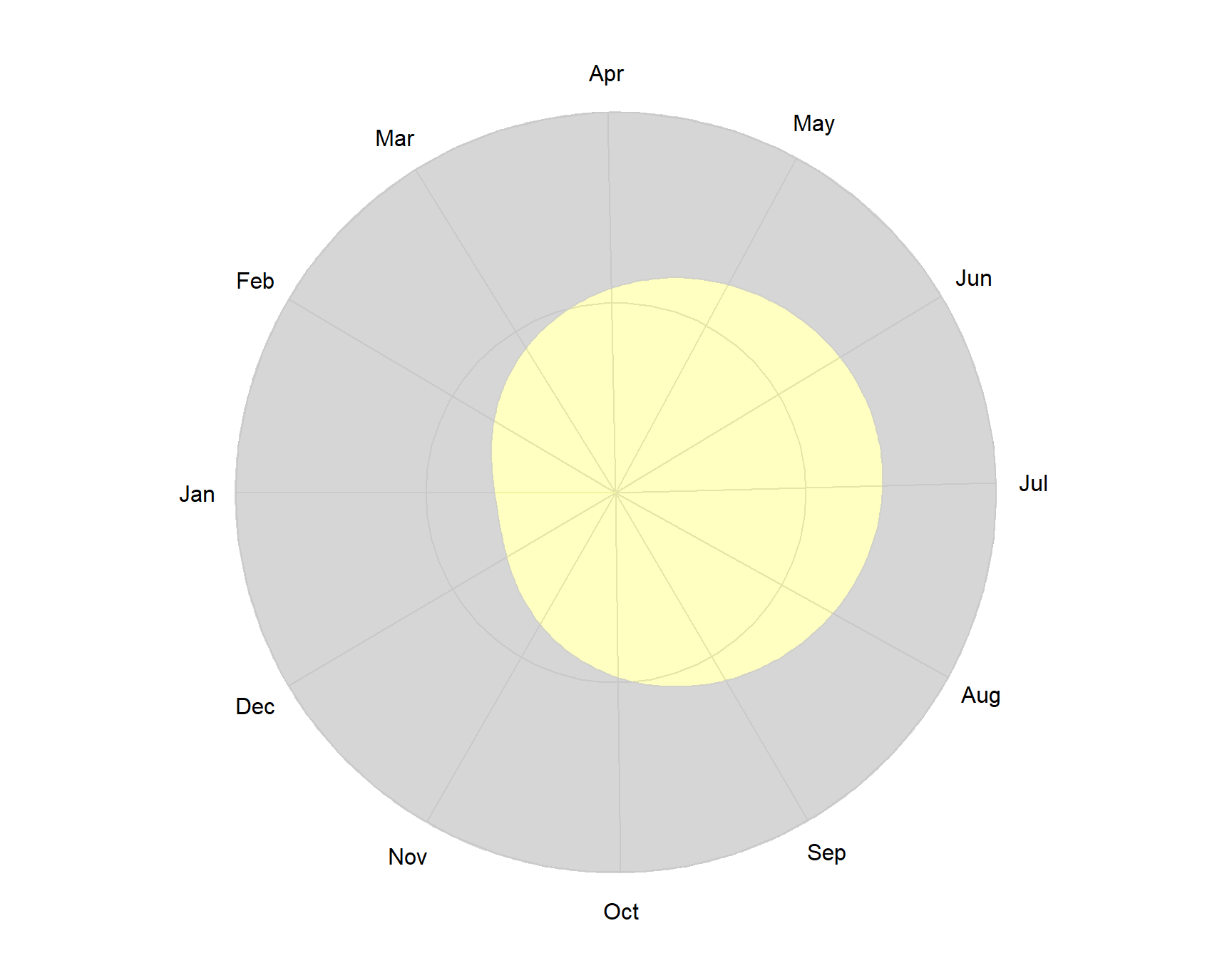
Figure 7.8: Example of a yearly plot

7.3 Lunar Cycles

7.4 Core and ring plots

These visualisations for cyclical data plot their information onto a circle with a radius of two units. It is possible to limit the plot either to the centre of the circle (a ‘core’ plot) or to the edge (a ‘ring plot’). These alternative forms may be more useful when these plots are used to visualise addition variables (7.7).

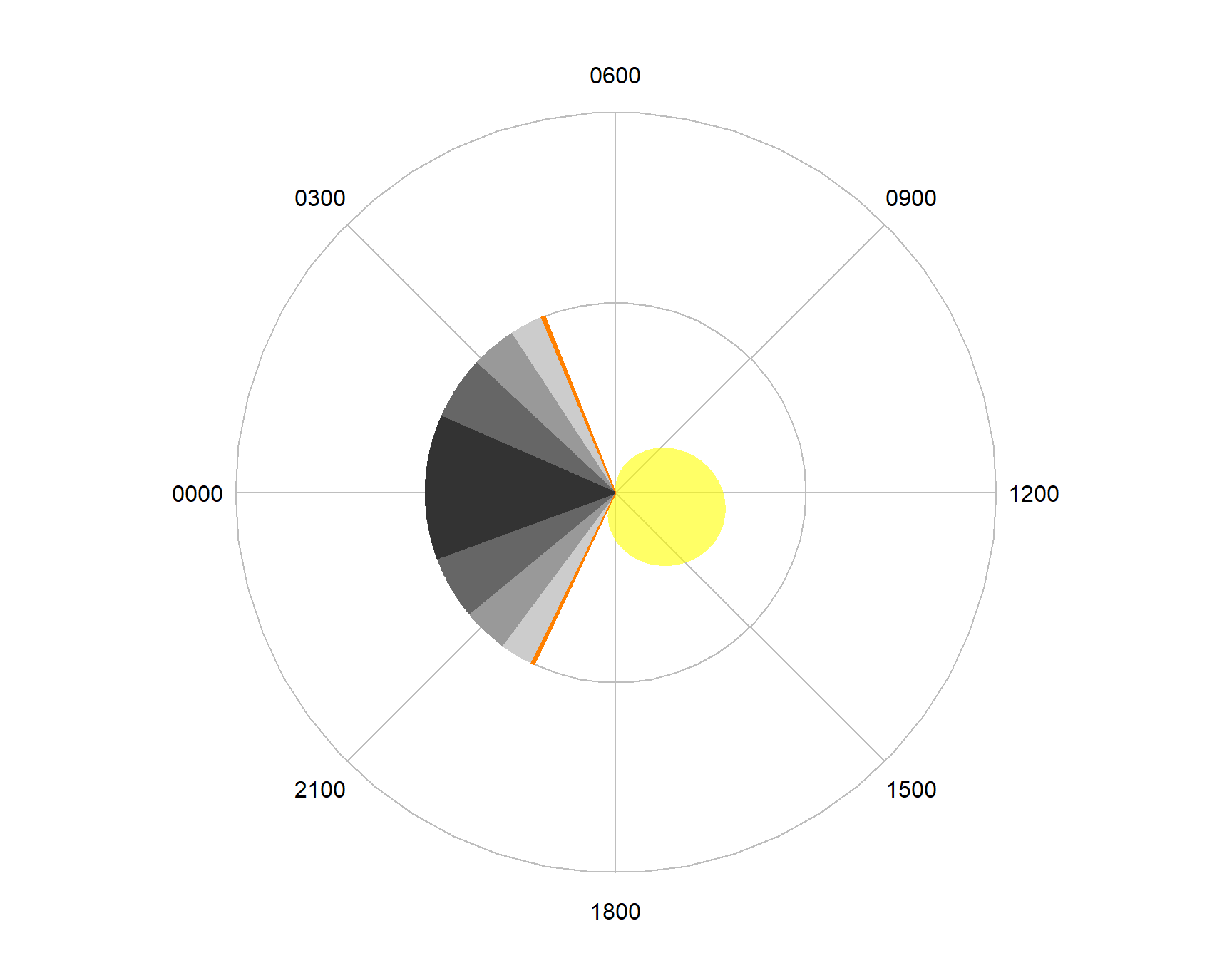
dielPlot("2022-08-08", lat=53, lon=0.1, limits=c(0,1))

Figure 7.9: A ‘core’ diel plot.

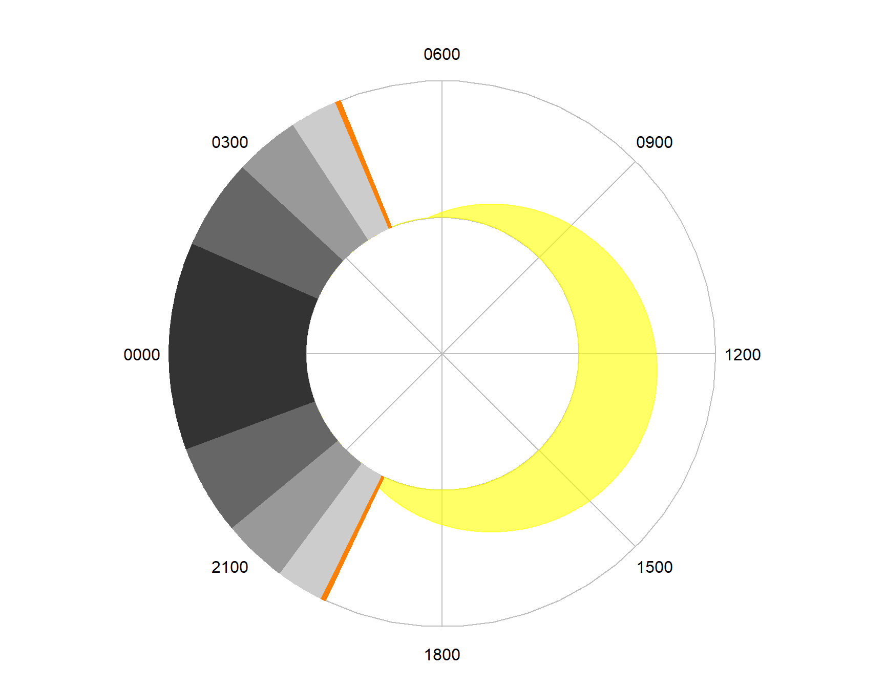
dielPlot("2022-08-08", lat=53, lon=0.1, limits=c(1,2))

Figure 7.10: A ‘ring’ diel plot.

7.5 Behind the scenes

7.5.1 `radialPolygon()`

The radialPolygon() function handles most of the plotting functionality for cyclical data in SonicScrewdriveR. It handles sectors, annuli, horizon plots and irregular polygons. It is used by the plotting functions such as dielPlot() and helper functions such as dielRings() to add data to cyclical plots.

For simple use cases, knowledge of the operation of radialPolygon() may not be needed. Several helper functions cover the most common uses. However, understanding how this function works will allow for far greater customisation of cyclical plots than would otherwise be possible.

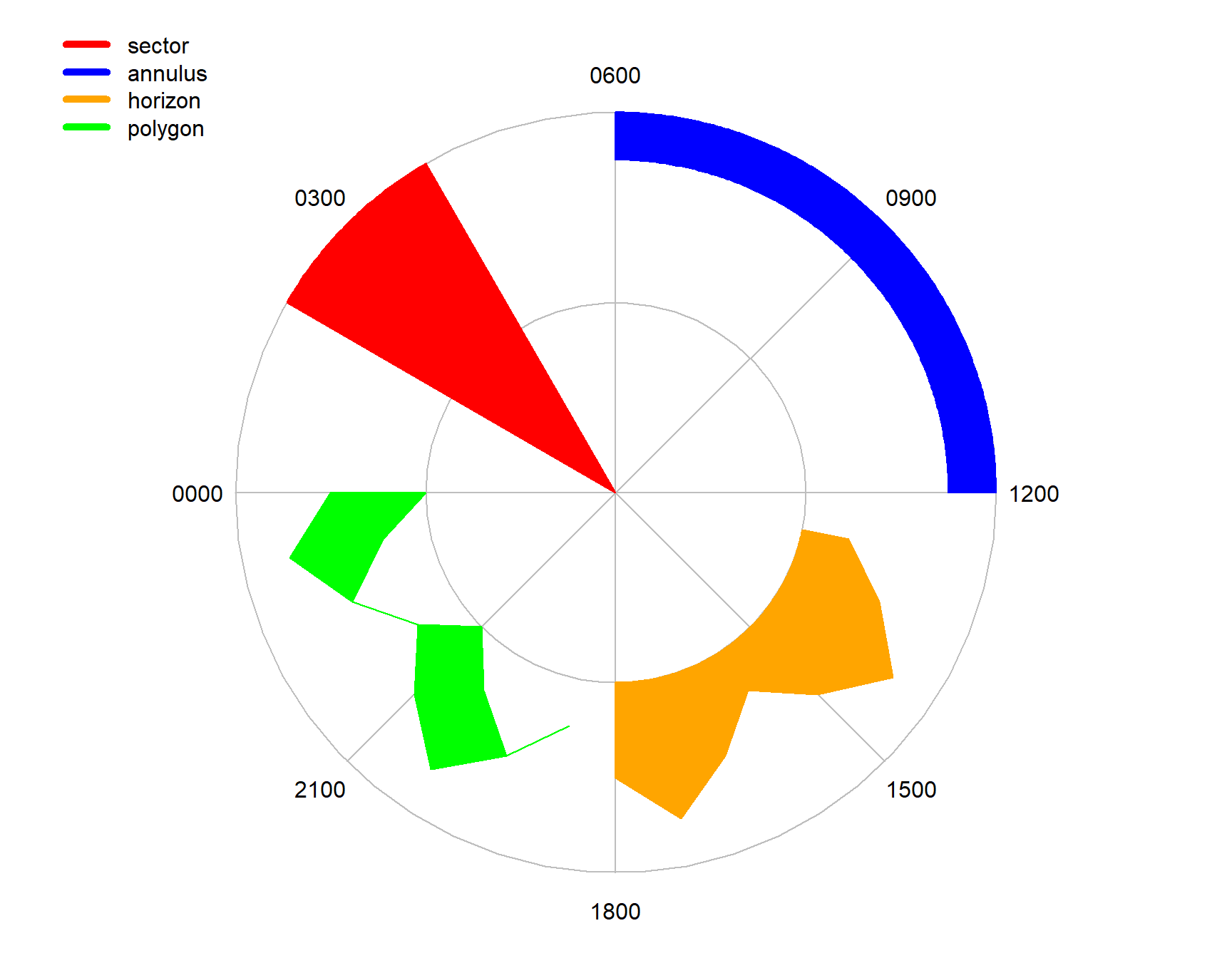
Figure 7.11: Types of radial polygon plot

The various types of plots are created by changing the angle and radius parameters to radialPolygon().

radialPolygon(angle1, angle2, radius1, radius2, col)

7.5.1.1 Orientation

Unlike traditional polar plots, diel and yearly plots start their periods on the left hand horizontal, and proceed clockwise. This orientation is assumed by radialPolygon(), although it may be modified (e.g. the parameters reverse=FALSE and rot=0 will plot using the standard conventions for polar coordinate systems.)

7.5.1.2 Sectors

A sector is a section of a circle defined by two radii and an arc between them. Sectors are used widely in the default settings of dielPlot() to plot the times of night and twilight.

emptyDiel()
radialPolygon(pi/6, 2*pi/3, 0, 2, col="red")

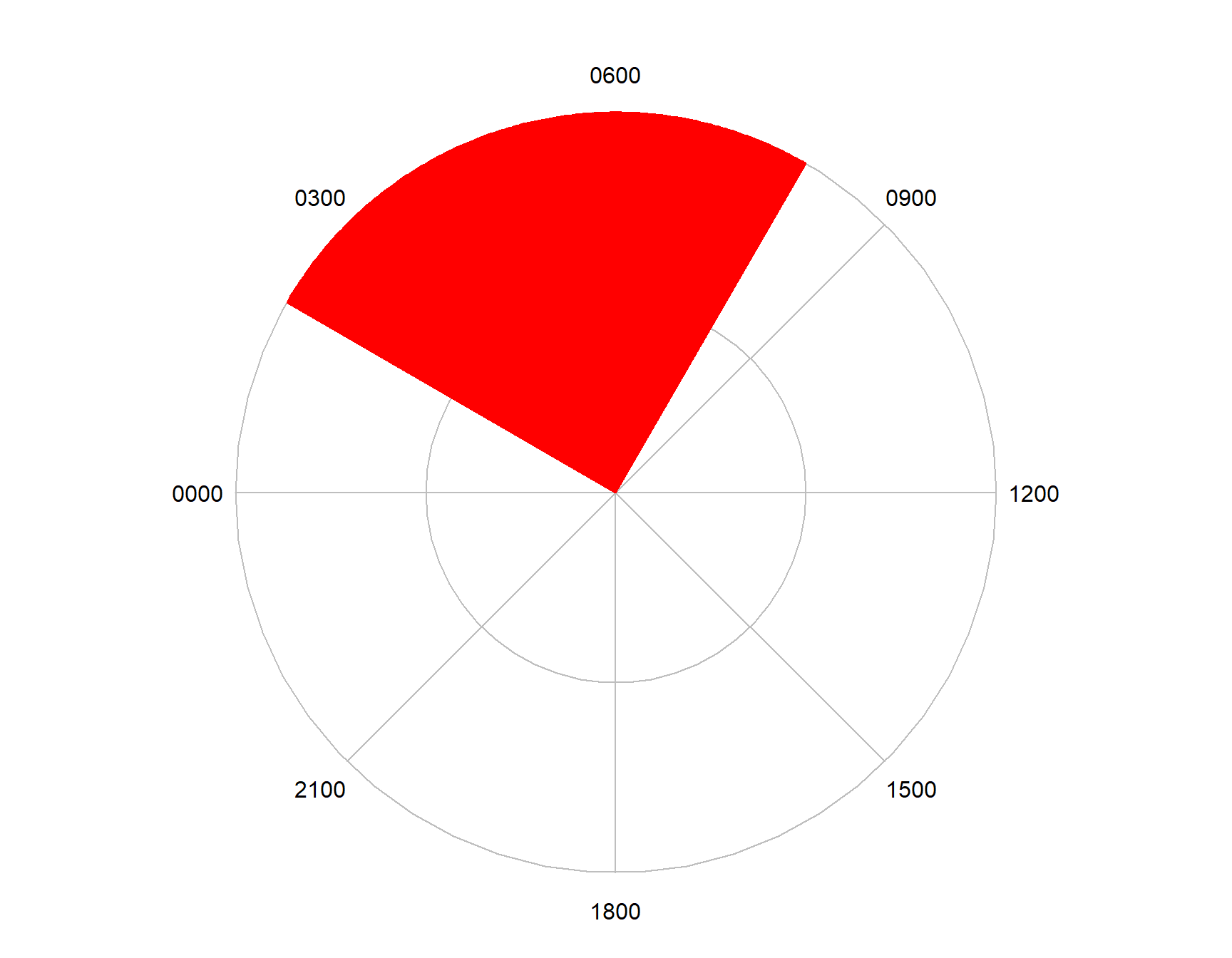
Figure 7.12: Plotting a sector

Reversing the angle arguments allows the complementary sector to be drawn.

emptyDiel()
radialPolygon(2*pi/3, pi/6, 0, 2, col="blue")

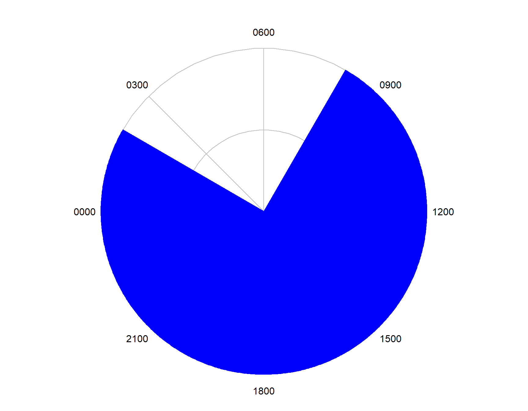
Figure 7.13: Plotting a sector

7.5.1.3 Annuli

An annulus is the region between two concentric circles. Annuli and annular sectors are generated by radialPolygon() when the parameter radius is greater than zero.

emptyDiel()
radialPolygon(0, 2*pi, 1.75, 2, col="blue")
radialPolygon(pi, 4*pi/3, 1, 1.5, col="red")
legend(
  -3,2.5,
  c("annulus", "annuluar sector"),
  col=c("blue", "red"),
  lty=1,
  lwd=5,
  bty = "n",
  cex = 1)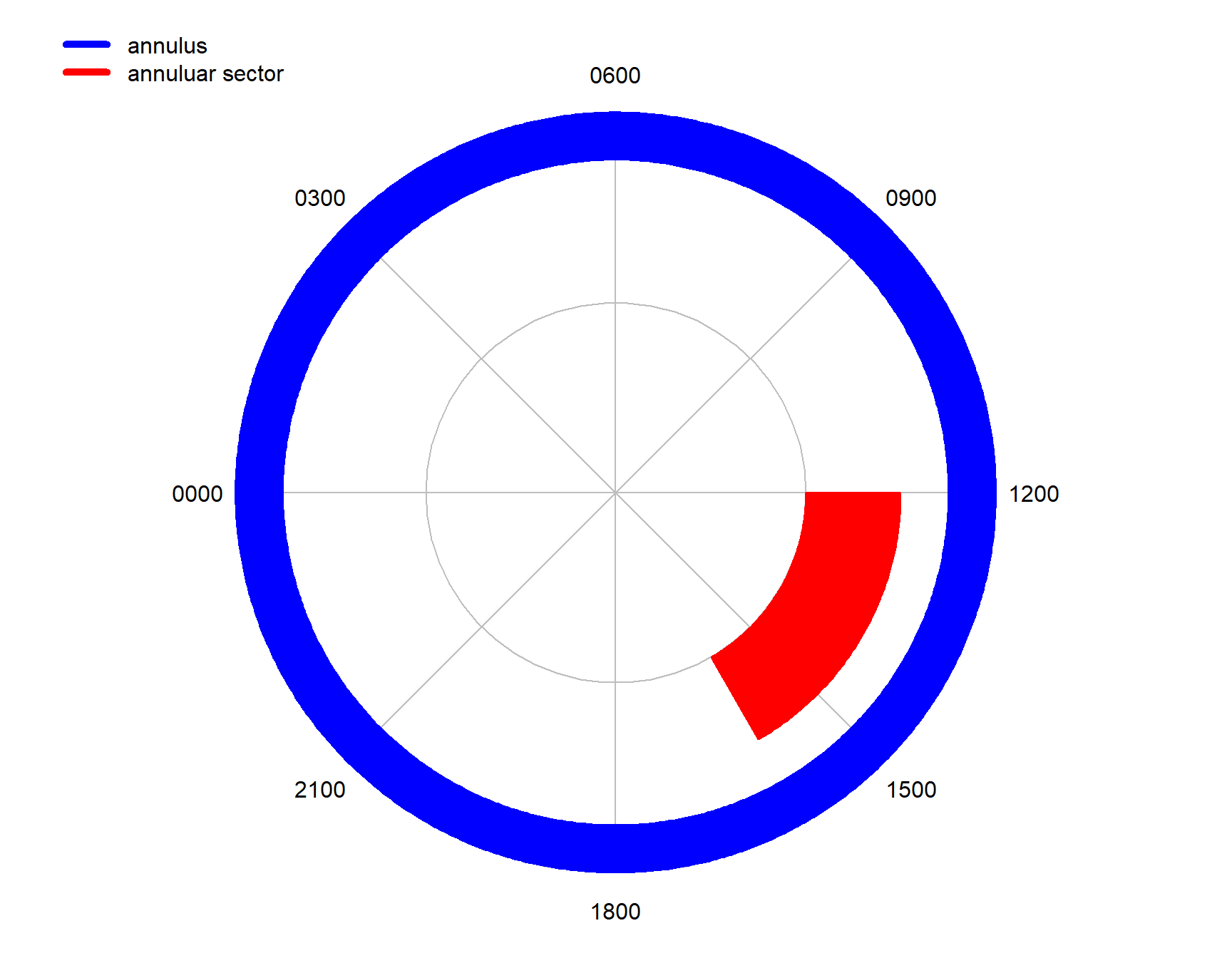

Figure 7.14: Plotting an annulus and an annular sector

7.5.1.4 Horizons

Horizons have one circular edge, and one that represents data, they are named as they often resemble a landscape or cityscape horizon. The example below uses a generated sine pattern to form the data edge.

library(tuneR)

angles <- (0:200)*pi/200 + pi/2
values <- 0.05*sine(10, samp.rate=201)@left

emptyDiel()
radialPolygon(NA,angles,0.5,1+values)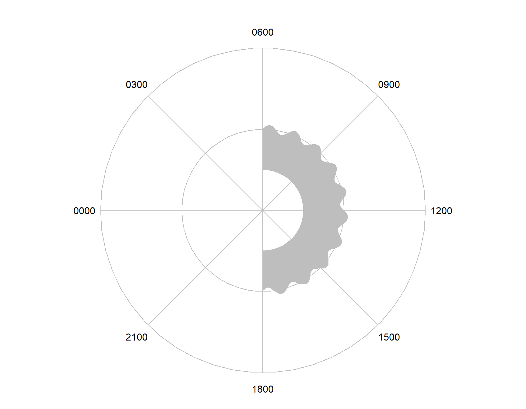

Figure 7.15: Plotting a horizon polygon.

Setting the first angle parameter to NA uses the range of the second to calculate the inner edge.

The inner edge can be used to show data by swapping the order of the angle and radius parameters.

library(tuneR)

angles <- (0:200)*pi/200 + pi/2
values <- 0.05*sine(10, samp.rate=201)@left

emptyDiel()
radialPolygon(angles,NA,1+values,2)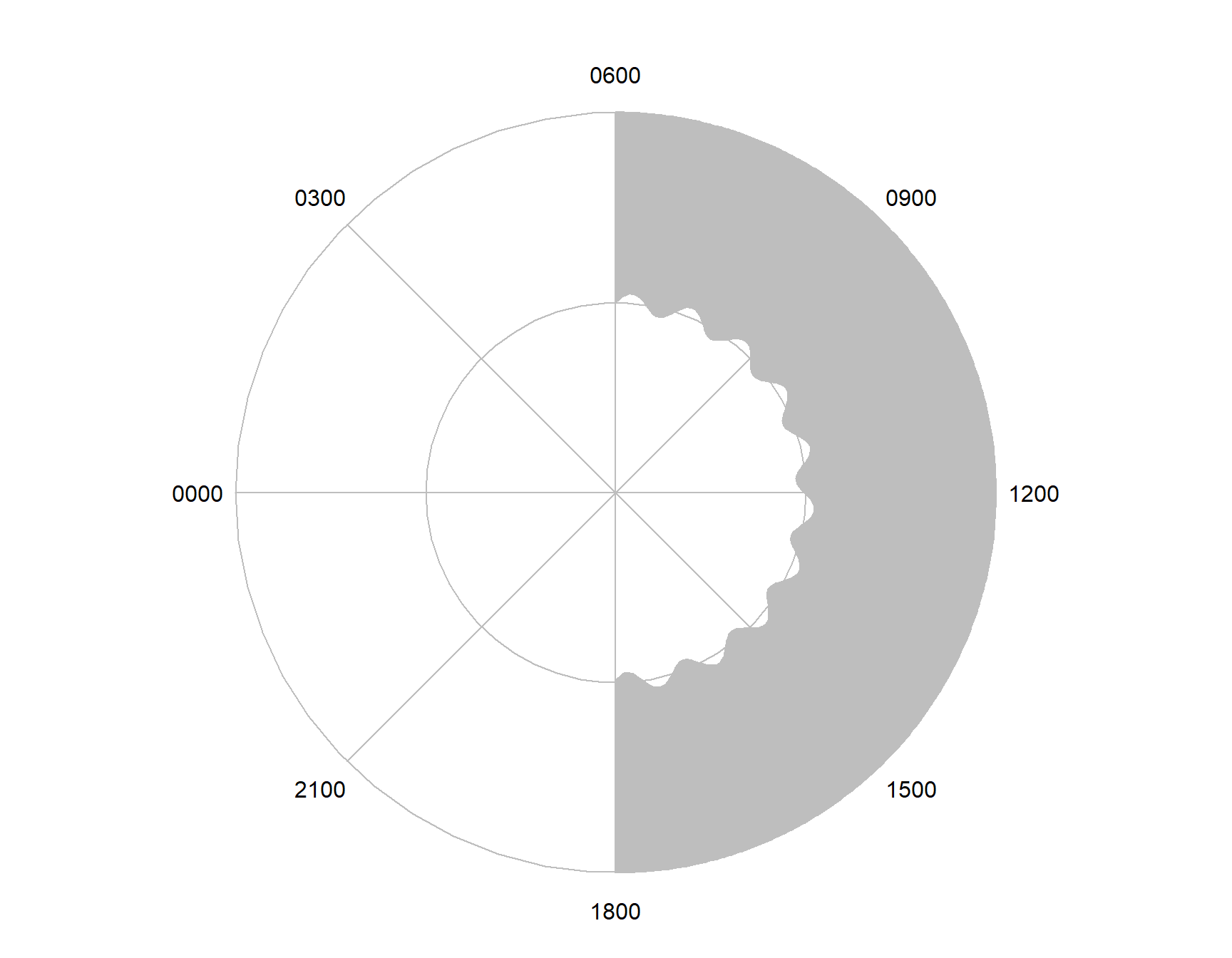

Figure 7.16: Plotting a horizon polygon.

The yearlyPlot() function uses two horizon plots, with a shared data edge.

7.5.1.5 Polygons

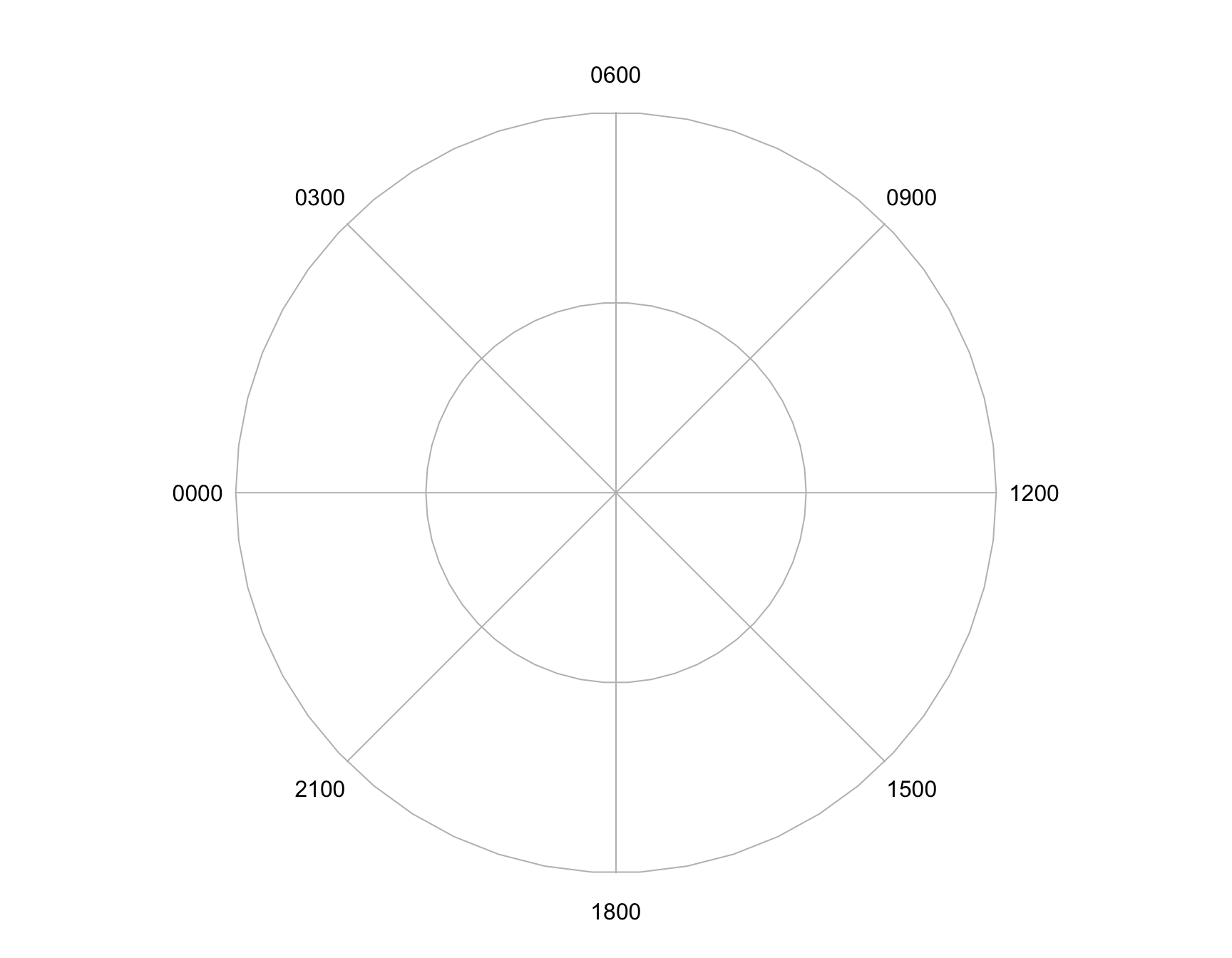
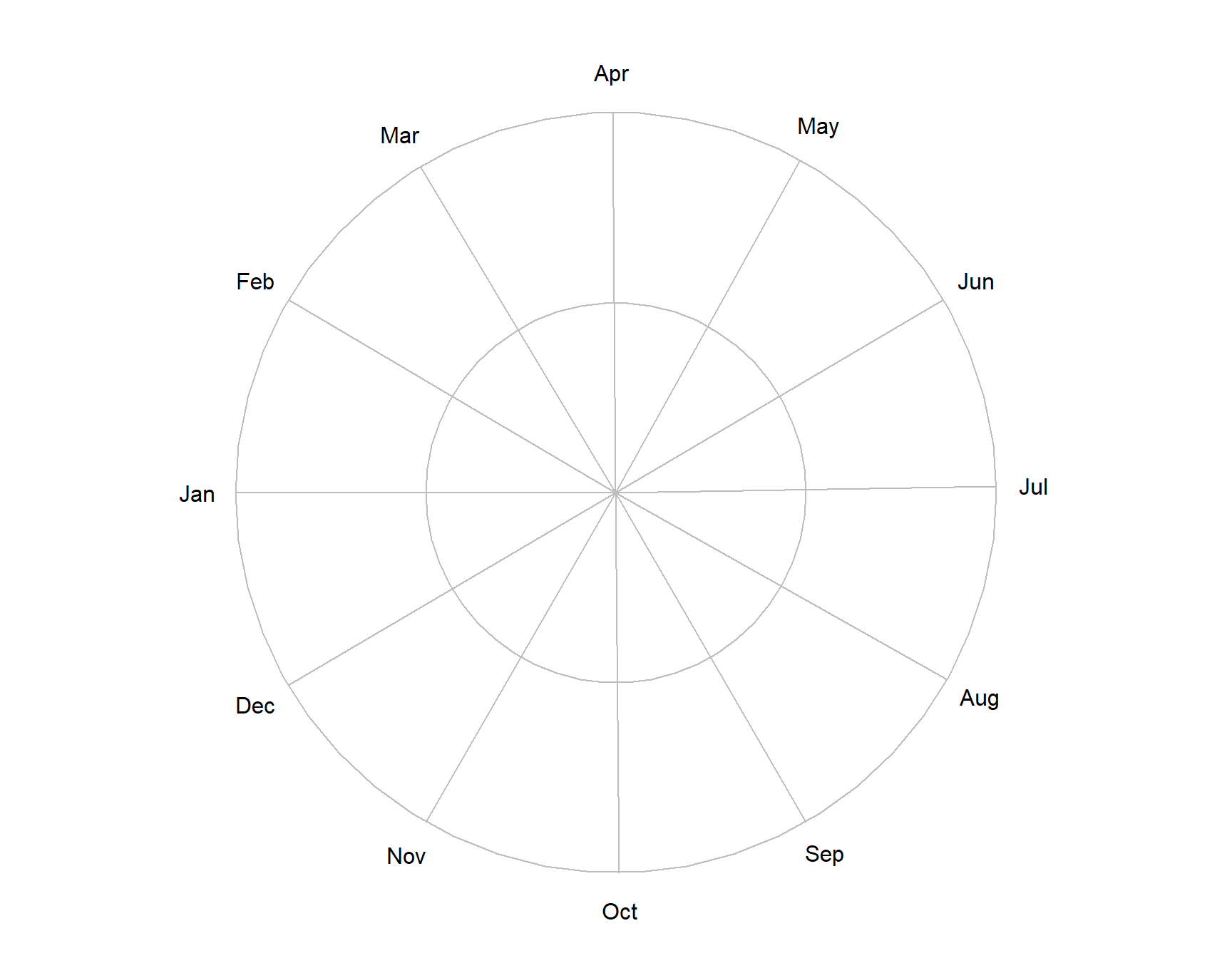
7.6 Empty plots

The uses of daily and yearly plots extend beyond linking data to earthly cycles. The following functions provide the basic coordinate system without any data plotted (these functions are used intenally by dielPlot() and yearlyPlot() to establish their coordinate system).

7.6.1 `emptyDiel()`

emptyDiel()

Figure 7.17: An empty dielPlot().

7.6.2 `emptyYearly()`

The emptyYearly() function takes an option year parameter that automatically adjusts the grid positions for leap years, although the visual effect is marginal.

emptyYearly(year=2000)

Figure 7.18: An empty yearlyPlot().

7.7 Adding data to the visualisation

7.7.1 Periodic data: rings

The ring functions (dielRing(),…) plot ring segments on top of a base cyclical plot. These rings are useful for showing typical periods of activity for a species, or events that happen continuously for a specified period of time.

By defaults the limits for the rings are 1,2 for use with a core type plot, but this can be changed by specifying the limits parameter to the ring function. Similarly, the plot legend may be removed with the paramater legend=FALSE.

7.7.1.1 `dielRings()`

names <- c("activity 1", "activity 2", "activity 3")
starts <- c("0600", "0900", "1500")
ends <- c("1200", "1700", "1900")
cols <- c("red", "green", "blue")

dielPlot("2022-08-08", lat=53, lon=0.1, limits=c(0,1))
dielRings(names, starts, ends, cols=cols)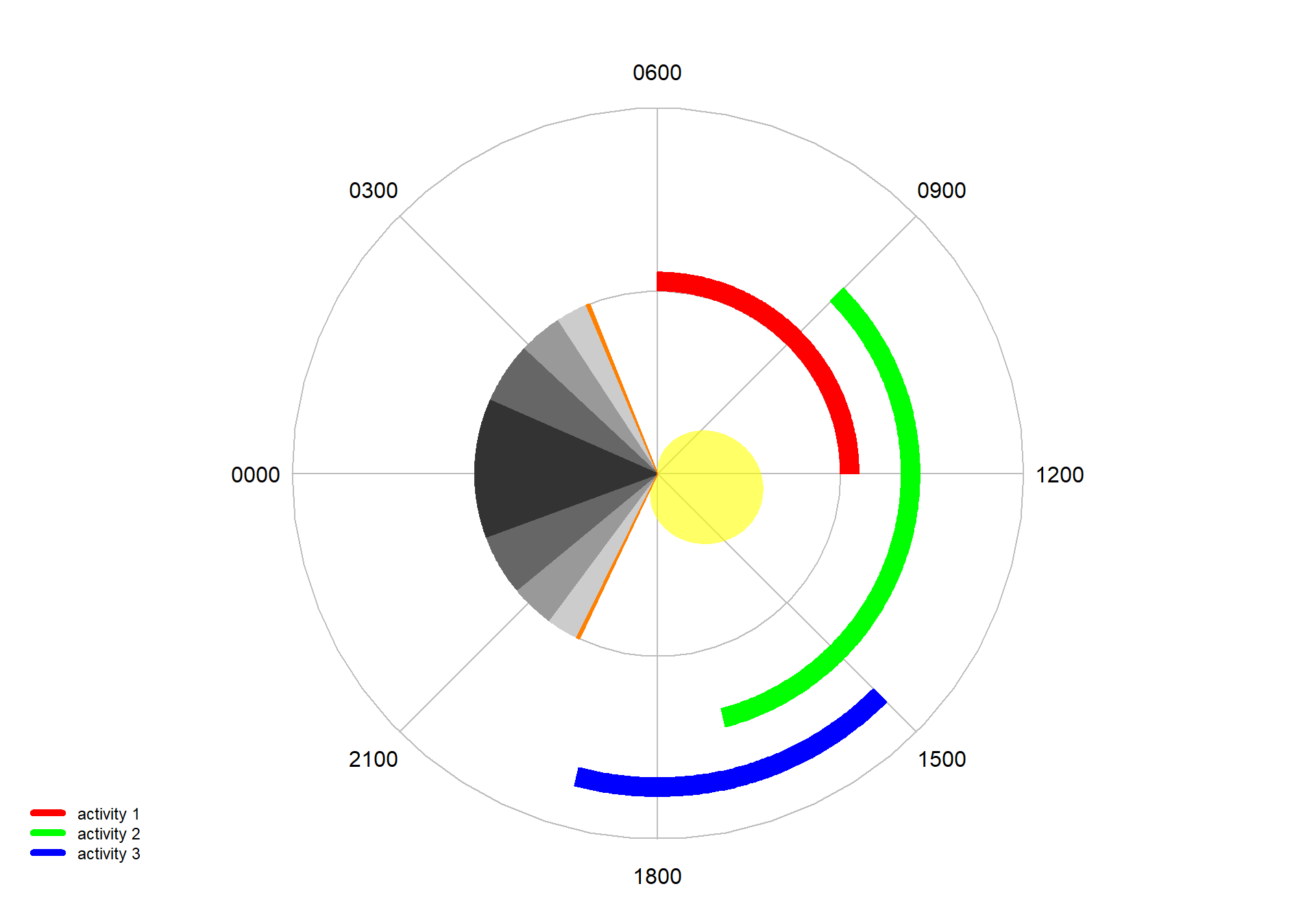

Figure 7.19: A ‘core’ diel plot with diel rings.

names <- c("activity 1", "activity 2", "activity 3")
starts <- c("0600", "0900", "1500")
ends <- c("1200", "1700", "1900")
cols <- c("red", "green", "blue")

dielPlot("2022-08-08", lat=53, lon=0.1, limits=c(1,2))
dielRings(names, starts, ends, cols=cols, limits=c(0,1))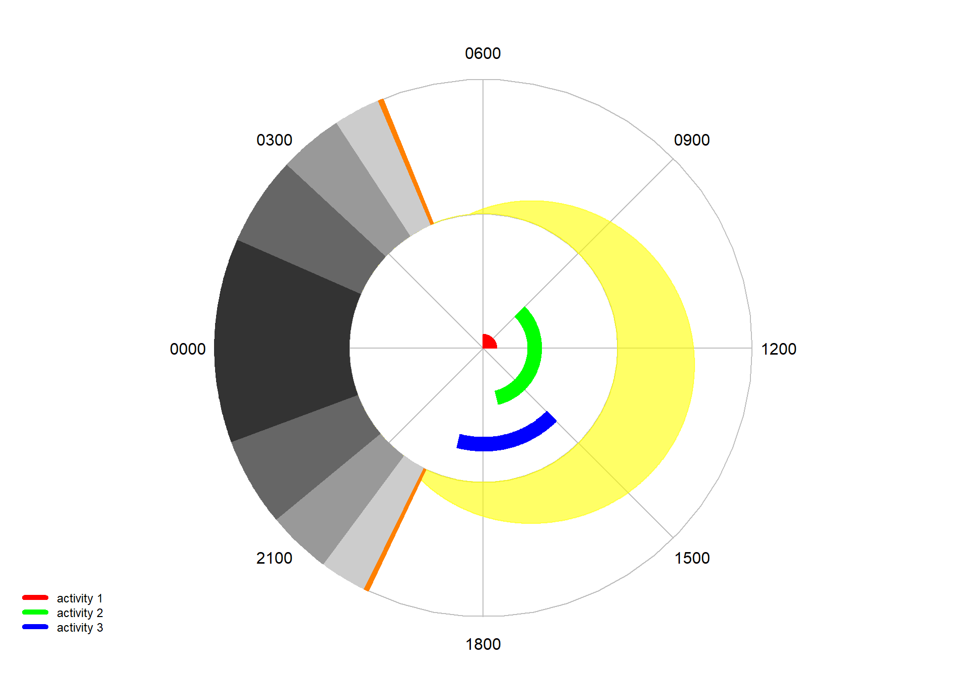

Figure 7.20: A ‘ring’ diel plot with diel rings.

7.7.2 Periodic data: horizons

In this example we will plot the average monthly minimum and maximum temperatures for Lyme Regis, UK onto a yearlyPlot(). This example introduces three small helper functions; yearlyLabels(), yearlyPositions() and circularise().

7.7.2.1 `yearlyLabels()` and `yearlyPositions`

These two functions are closely related, and used internally by SonicScrewdriveR to label a yearly plot.

yearlyLabels()

##  [1] "Jan" "Feb" "Mar" "Apr" "May" "Jun" "Jul" "Aug" "Sep" "Oct" "Nov" "Dec"

The related yearlyPositions() gives angular positions for the data around the plot (in radians).

yearlyPositions(year=2022)

##  [1] 0.0000000 0.5336404 1.0156382 1.5492786 2.0657048 2.5993452 3.1157713
##  [8] 3.6494117 4.1830521 4.6994783 5.2331187 5.7495449

The temperature data we have for Lyme Regis is monthly, however we would like to plot the values at the middle of the respective month. For this we add the parameter format="mid-month" to get the appropriate radial angles.

yearlyPositions(year=2022, format="mid-months")

##  [1] 0.2668202 0.7746393 1.2824584 1.8074917 2.3325250 2.8575582 3.3825915
##  [8] 3.9162319 4.4412652 4.9662985 5.4913318 5.9733296

If we now plot this data we see that the output is not quite a complete ring or horizon data as we might have expected.

# Temperature data for Lyme Regis
t_min <- c(3, 2.7, 3.4, 5.2, 8.2, 11.2, 13.1, 13, 14.4, 9.2, 5.8, 3.8)
t_max <- c(7.9,8, 9.8, 12.4, 15.4, 18.2, 20.1, 19.5, 17.8, 14.4, 10.6, 8.4)

# Scale the data
sf <- max(t_max)
t_min <- t_min/sf
t_max <- t_max/sf

angles <- yearlyPositions(format="mid-months")

yearlyPlot(lat=50.7, lon=-2.9)
radialPolygon(angles, angles, t_min, t_max, col="orange")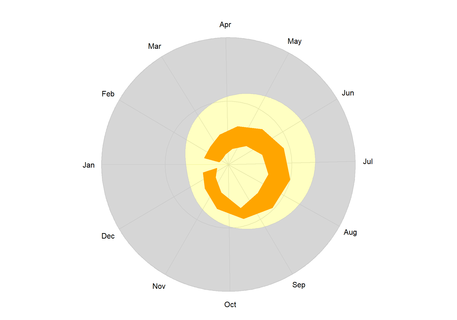

Figure 7.21: Horizon data plot without circularise().

7.7.2.2 `circularise()`

In order to join the horizons into a complete ring we can use the circularise() function on the angle and temperature vectors.

# Temperature data for Lyme Regis
t_min <- c(3, 2.7, 3.4, 5.2, 8.2, 11.2, 13.1, 13, 14.4, 9.2, 5.8, 3.8)
t_max <- c(7.9,8, 9.8, 12.4, 15.4, 18.2, 20.1, 19.5, 17.8, 14.4, 10.6, 8.4)

# Scale the data
sf <- max(t_max)
t_min <- t_min/sf
t_max <- t_max/sf

angles <- yearlyPositions(format="mid-months")

# Circularise
t_min <- circularise(t_min)
t_max <- circularise(t_max)
angles <- circularise(angles)

yearlyPlot(lat=50.7, lon=-2.9)
radialPolygon(angles, angles, t_min, t_max, col="orange")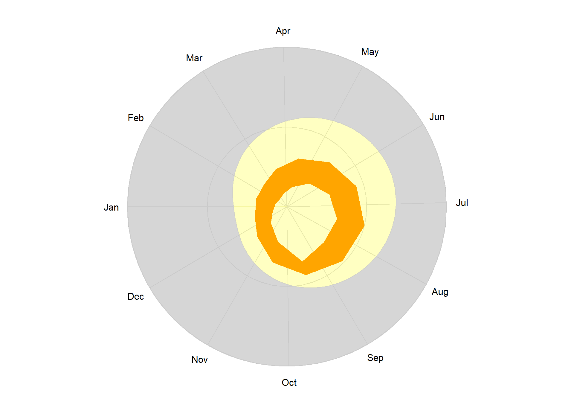

Figure 7.22: Horizon data plot with circularise().

7.7.3 Helper functions

7.7.3.1 `dielFraction()`

The dielFraction() function is used to convert a POSIX time, or a time in HHMM string format, into a radial fraction. This function is called by dielPlot() and dielRings(). By default the output is multiplied by 2π to output a position round a circle.

time <- Sys.time()
print(time)

## [1] "2024-01-24 19:11:25 GMT"

frac <- dielFraction(time)
print(frac)

## [1] 5.024044

The raw fraction can be specified using the parameter unit="fraction".

time <- Sys.time()
print(time)

## [1] "2024-01-24 19:11:25 GMT"

frac <- dielFraction(time, unit="fraction")
print(frac)

## [1] 0.7996016

7.7.3.2 `yearlyFraction()`

Similarly to dielFraction(), yearlyFraction() by default returns a fraction of a cycle. It can take either a number representing a day of the year, or an object that can be coerced into POSIXlt format.

frac <- yearlyFraction(31, input="day")
print(frac)

## [1] 0.5336404

date <- Sys.Date()
print(date)

## [1] "2024-01-24"

frac <- yearlyFraction(date, input="POSIXlt")
print(frac)

## [1] 0.3959267

7.8 Interactive Plots

These plots can be used to create Shiny apps

shiny-diel is an example that shows diel plots for a number of locations, and can be animated using the play button under the date slider.

References

Baker, Ed. 2021. SonicScrewdriveR. https://cran.r-project.org/package=sonicscrewdriver.

Lemon, J. 2006. “Plotrix: A Package in the Red Light District of r.” R-News 6 (4): 8–12.

Thieurmel, Benoit, and Achraf Elmarhraoui. 2019. Suncalc: Compute Sun Position, Sunlight Phases, Moon Position and Lunar Phase. https://CRAN.R-project.org/package=suncalc.